Durbin watson tables

The Durbin-Watson test statistic tests the null hypothesis that the residuals from an

ordinary least-squares regression are not autocorrelated against the alternative that the

residuals follow an AR1 process. The Durbin-Watson statistic ranges in value from 0

to 4. A value near 2 indicates non-autocorrelation; a value toward 0 indicates positive

autocorrelation; a value toward 4 indicates negative autocorrelation.

Because of the dependence of any computed Durbin-Watson value on the

associated data matrix, exact critical values of the Durbin-Watson statistic are not

tabulated for all possible cases. Instead, Durbin and Watson established upper and

lower bounds for the critical values. Typically, tabulated bounds are used to test the

hypothesis of zero autocorrelation against the alternative of positive first-order

autocorrelation, since positive autocorrelation is seen much more frequently in

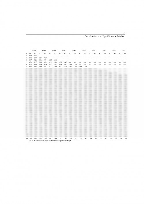
practice than negative autocorrelation. To use the table, you must cross-reference the

sample size against the number of regressors, excluding the constant from the count

of the number of regressors.

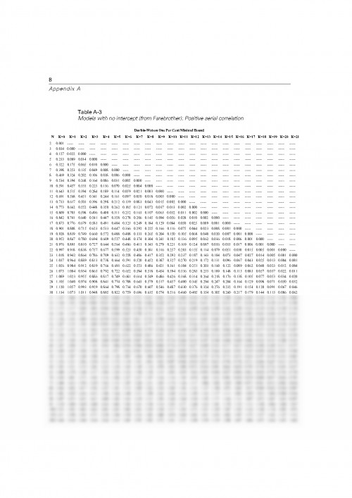
The conventional Durbin-Watson tables are not applicable when you do not have

a constant term in the regression. Instead, you must refer to an appropriate set of

Durbin-Watson tables. The conventional Durbin-Watson tables are also not

applicable when a lagged dependent variable appears among the regressors. Durbin

has proposed alternative test procedures for this case.

Statisticians have compiled Durbin-Watson tables from some special cases,

including:

- Regressions with a full set of quarterly seasonal dummies.

- Regressions with an intercept and a linear trend variable (CURVEFIT

MODEL=LINEAR).

- Regressions with a full set of quarterly seasonal dummies and a linear trend

variable.

Appendix A

In addition to obtaining the Durbin-Watson statistic for residuals from REGRESSION,

you should also plot the ACF and PACF of the residuals series. The plots might suggest

either that the residuals are random, or that they follow some ARMA process. If the

residuals resemble an AR1 process, you can estimate an appropriate regression using

the AREG procedure. If the residuals follow any ARMA process, you can estimate an

appropriate regression using the ARIMA procedure.

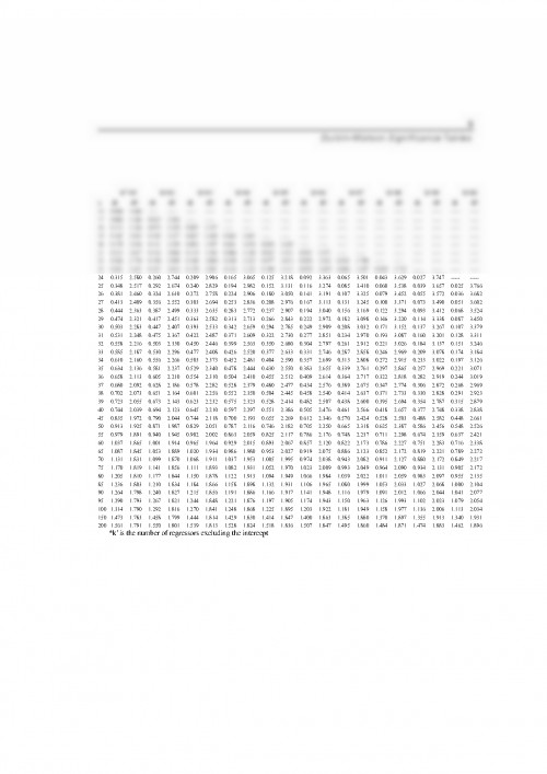
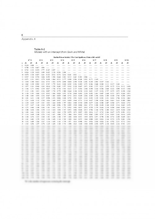
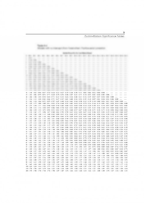
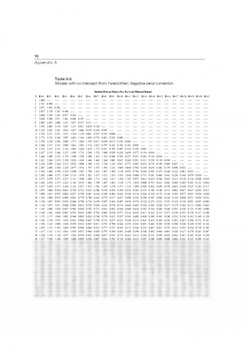
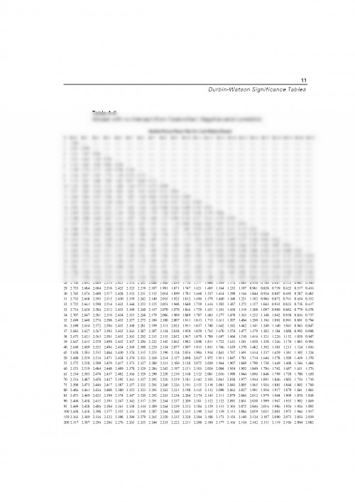
In this appendix, we have reproduced two sets of tables. Savin and White (1977)

present tables for sample sizes ranging from 6 to 200 and for 1 to 20 regressors for

models in which an intercept is included. Farebrother (1980) presents tables for sample

sizes ranging from 2 to 200 and for 0 to 21 regressors for models in which an intercept

is not included.

Let's consider an example of how to use the tables. In Chapter 9, we look at the

classic Durbin and Watson data set concerning consumption of spirits. The sample size

is 69, there are 2 regressors, and there is an intercept term in the model. The Durbin-

Watson test statistic value is 0.24878. We want to test the null hypothesis of zero

autocorrelation in the residuals against the alternative that the residuals are positively

autocorrelated at the 1% level of significance. If you examine the Savin and White

tables (Table A.2 and Table A.3), you will not find a row for sample size 69, so go to

the next lowest sample size with a tabulated row, namely N=65. Since there are two

regressors, find the column labeled k=2. Cross-referencing the indicated row and

column, you will find that the printed bounds are dL = 1.377 and dU = 1.500. If the

observed value of the test statistic is less than the tabulated lower bound, then you

should reject the null hypothesis of non-autocorrelated errors in favor of the hypothesis

of positive first-order autocorrelation. Since 0.24878 is less than 1.377, we reject the

null hypothesis. If the test statistic value were greater than dU, we would not reject the

null hypothesis.